Optimization Procedure
With the presence of numerous variables in a complex LP problem, the optimal solution can only be achieved by the delicate trade-off in allocating the production of products to the manufacturing plants in the way to minimize the overall logistics costs. For an LP problem of a realistic size, the size of the search space and the number of feasible solutions could be extremely large. The principle of GA optimization differs from most traditional optimization methods in that GA is capable of handling large search spaces easily [59,68,69].
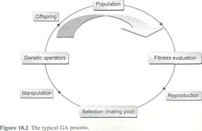
In a typical type of GA (refer to Figure 18.2), the possible solutions of the problem are represented by chromosomes. Every chromosome is coded in the way to contain the potential solution to the problem. This process is called chromosome representation and forms the main difference between various GA models. In the first step of the GA process, a population of chromosomes is created with a group of randomly generated solutions (chromosomes). Then, all individuals in the population are evaluated by scoring them based on how fit they are (i.e., a fitness value for each chromosome). Following this, multiple individuals are randomly selected from the population to produce offspring through the application of genetic operators (generally includes crossover operator and mutation operators). The generated offspring form the new generation. Fitness values are evaluated again for the new generation. Based on the concept of natural evolution, this process evolves toward a belter solution in consecutive generations. The reproduction process (i.e., scoring, crossover, and mutation) is repeated until a suitable solution is found or the termination criteria are satisfied. This process is illustrated in Figure 18.2.
For the proposed case problem in this chapter, the developed cost function in Section 18.4 (i.e., objective function in Eqn (18.1)) acts as the fitness function in
|
the GA process. It has been a common approach in solving LP problems to define the fitness function equal to the objective function, which in many cases is also the c0st function [49,74,75,78J. In this case, the chromosome with the lowest fitness value signifies the fittest chromosome. To simplify the coding process, a linear chromosome representation is adopted for the presented case study. In this way, all 0f the decision variables (see Section 18.4) are located along a straight chromosome in which each gene of the chromosome accommodates the real value of a variable.
A multipoint crossover operator is employed for the proposed GA model. In a single-point crossover operator, a crossover point is randomly selected between the first and last bits of the parents' chromosomes. Parents 1 and 2 pass their binary codes from the left of the crossover point to offspring 1 and 2, respectively. Then the binary codes in the right of the crossover point of parent 1 and parent 2 go to offspring 2 and offspring 1, respectively. The number of randomly selected crossover points determines the type of crossover used: single point, two point, or multiple point. In terms of chromosome maintenance, the destructive effects of a multipoint crossover may lead to more exploration rather than exploitation in chromosomes, whereas having a small number of crossover points contributes to more exploitation than exploration [ 12].
A simple flip nonuniform mutation is adopted as the background operator in the sense that it helps GA find the solutions that crossover alone might not encounter. A mutation operator alters a certain percentage of the bits (genes) in a chromosome. This can stop GA from early convergence and ensure the feasibility of the developed offspring by maintaining diversity in the population [ 12]. Crossover rate and mutation rate (e.g., the proportion of chromosomes in the mating pool on which the crossover and mutation operator will apply) is to be determined experimentally (i.e., trial and error practice).
It is always difficult to prove the convergence to the optimal solution in the optimization of complex problems. Therefore, a termination point is generally set to stop the process. A multiple termination condition is adopted in the proposed GA procedure in this chapter: (1) stop by limiting the number of iterations or generations and (2) stop when minimal change in fitness value is observed in consecutive generations.